T-Test

A statistical examination of two population means. A two-sample t-test examines whether two samples are different and is commonly used when the variances of two normal distributions are unknown and when an experiment uses a small sample size. For example, a t-test could be used to compare the average floor routine score of the U.S. women's Olympic gymnastic team to the average floor routine score of China's women's team.

Descriptive Statistics

Descriptive statistics are used to describe the basic features of the data in a study. They provide simple summaries about the sample and the measures. Together with simple graphics analysis, they form the basis of virtually every quantitative analysis of data.

Descriptive statistics are typically distinguished from inferential statistics. With descriptive statistics you are simply describing what is or what the data shows. With inferential statistics, you are trying to reach conclusions that extend beyond the immediate data alone. For instance, we use inferential statistics to try to infer from the sample data what the population might think. Or, we use inferential statistics to make judgments of the probability that an observed difference between groups is a dependable one or one that might have happened by chance in this study. Thus, we use inferential statistics to make inferences from our data to more general conditions; we use descriptive statistics simply to describe what's going on in our data.

Other Effective Sampling Methods

Review: Simple Random Sampling

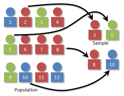
Do you remember how simple random sampling works? Visually, it's just numbering each individual and randomly selecting a certain number of them. Here's the image we used in the previous section:

Stratified Sampling

Stratified sampling is different. With this technique, we separate the population using some characteristic, and then take a proportional random sample from each.

A stratified sample is obtained by separating the population into non-overlapping groups called strata and then obtaining a proportional simple random sample from each group. The individuals within each group should be similar in some way.

Visually, it might look something like the image below. With our population, we can easily separate the individuals by color.

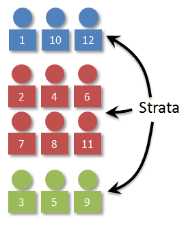
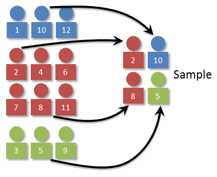
Once we have the strata determined, we need to decide how many individuals to select from each stratum. (Man, that's a weird word!) The key here is that the number selected should beproportional. In our case, 1/4 of the individuals in the population are blue, so 1/4 of the sample should be blue as well. Working things out, we can see that a stratified (by color) random sample of 4 should have 1 blue, 1 green, and 2 reds.

Example 1

One easy example using a stratified technique would be a sampling of people at ECC. To make sure that a sufficient number of students, faculty, and staff are selected, we would stratify all individuals by their status - students, faculty, or staff. (These are the strata.) Then, a proportional number of individuals would be selected from each group.

Systematic Sampling

A systematic sample is obtained by selecting every kth individual from the population. The first individual selected corresponds to a random number between 1 and k.

So to use systematic sampling, we need to first order our individuals, then select every kth. (More on how to select k in a bit.)

In our example, we want to use 3 for k? Can you see why? Think what would happen if we used 2 or 4.

For our starting point, we pick a random number between 1 and k. For our visual, let's suppose that we pick 2. The individuals sampled would then be 2, 5, 8, and 11.

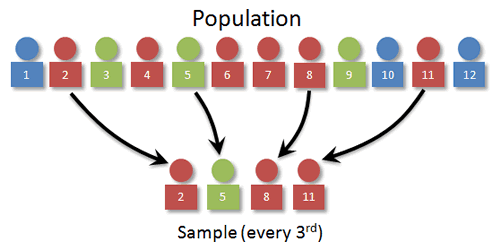
In general we find k by taking N/n and rounding down to the nearest integer.

Example 2

Systematic sampling works well when the individuals are already lined up in order. In the past, students have often used this method when asked to survey a random sample of ECC students. Since we don't have access to the complete list, just stand at a corner and pick every 10th* person walking by.

* Of course, choosing 10 here is just an example. It would depend on the number of students typically passing by that spot and what sample size was needed.

Cluster Sampling

Cluster sampling is often confused with stratified sampling, because they both involve "groups". In reality, they're very different. In stratified sampling, we split the population up into groups (strata) based on some characteristic.

So to use systematic sampling, we need to first order our individuals, then select every kth. (More on how to select k in a bit.)

In our example, we want to use 3 for k? Can you see why? Think what would happen if we used 2 or 4.

For our starting point, we pick a random number between 1 and k. For our visual, let's suppose that we pick 2. The individuals sampled would then be 2, 5, 8, and 11.

In general we find k by taking N/n and rounding down to the nearest integer.

For another take, watch this YouTube video:

Example 2

Systematic sampling works well when the individuals are already lined up in order. In the past, students have often used this method when asked to survey a random sample of ECC students. Since we don't have access to the complete list, just stand at a corner and pick every 10th* person walking by.

* Of course, choosing 10 here is just an example. It would depend on the number of students typically passing by that spot and what sample size was needed.

Cluster Sampling

Cluster sampling is often confused with stratified sampling, because they both involve "groups". In reality, they're very different. In stratified sampling, we split the population up into groups (strata) based on some characteristic.

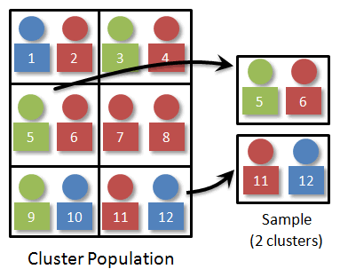
A cluster sample is obtained by selecting all individuals within a randomly selected collection or group of individuals.

In essence, we use cluster sampling when our population is already broken up into groups (clusters), and each cluster represents the population. That way, we just select a certain number of clusters.

With our visual, let's suppose the 12 individuals are paired up just as they were sitting in the original population.

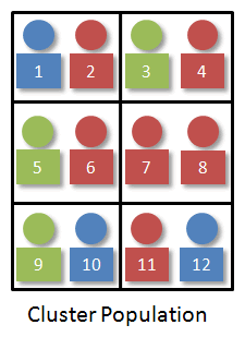
Since we want a random sample of size four, we just select two of the clusters. We would number the clusters 1-6 and use technology to randomly select two random numbers. It might look something like this:

Example 3

One situation where cluster sampling would apply might be in manufacturing. Suppose your company makes light bulbs, and you'd like to test the effectiveness of the packaging. You don't have a complete list, so simple random sampling doesn't apply, and the bulbs are already in boxes, so you can't order them to use systematic. And all the bulbs are essentially the same, so there aren't any characteristics with which to stratify them.

To use cluster sampling, a quality control inspector might select a certain number of entire boxes of bulbs and test each bulb within those boxes. In this case, the boxes are theclusters.

Convenience Sampling

Other methods do exist for finding samples of populations. In fact, you've seen some already. Probably the most common is the so-called convenience sample. Convenience samples are just what they sound like - convenient. Unfortunately, they're rarely representative. Think of the radio call-in show, those people in the shopping malls trying to survey you about your purchasing habits, or even the voting on American Idol!

Here's a specific example. It's a poll on beliefnet.com, titled "What Evangelicals Want". All online polls use, by nature, convenience sampling. According to the article, "The poll was promoted on Beliefnet’s web site and through its newsletters." Only those evangelicals who visit this particular web site and actually answer the survey are included. Beware any poll result taken with convenience sampling.

Multistage Sampling

Often one technique isn't possible, so many professional polling agencies use a technique called multistage sampling. The strategy is relatively self-explanatory - two or more sampling techniques are used.

For example, consider the light-bulb example we looked at earlier with cluster sampling. Let's suppose that the bulbs come off the assembly line in boxes that each contain 20 packages of four bulbs each. One strategy would be to do the sample in two stages:

Stage 1: A quality control engineer removes every 200th box coming off the line. (The plant produces 5,000 boxes daily. (This is systematic sampling.)

Stage 2: From each box, the engineer then samples three packages to inspect. (This is an example of cluster sampling.)

The US Census also uses multistage sampling. If you haven't already (you should have!), read Section 1.4 in your text for more details.

Summary

Here's a visual summary of the four main sampling strategies:

Simple Random:
Stratified:
Systematic: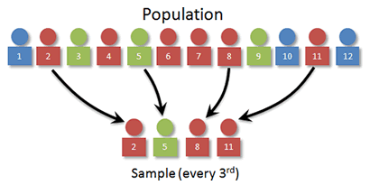
Cluster:

Confidence Intervals

A confidence interval gives an estimated range of values which is likely to include an unknown population parameter, the estimated range being calculated from a given set of sample data.

What is Hypothesis Testing?

A statistical hypothesis is an assumption about a population parameter. This assumption may or may not be true. Hypothesis testing refers to the formal procedures used by statisticians to accept or reject statistical hypotheses.

Statistical Hypotheses

The best way to determine whether a statistical hypothesis is true would be to examine the entire population. Since that is often impractical, researchers typically examine a random sample from the population. If sample data are not consistent with the statistical hypothesis, the hypothesis is rejected.

There are two types of statistical hypotheses.

• Null hypothesis. The null hypothesis, denoted by H₀, is usually the hypothesis that sample observations result purely from chance.
  
• Alternative hypothesis. The alternative hypothesis, denoted by H₁ or H_a, is the hypothesis that sample observations are influenced by some non-random cause.

For example, suppose we wanted to determine whether a coin was fair and balanced. A null hypothesis might be that half the flips would result in Heads and half, in Tails. The alternative hypothesis might be that the number of Heads and Tails would be very different. Symbolically, these hypotheses would be expressed as

H₀: P = 0.5
H_a: P ≠ 0.5

Suppose we flipped the coin 50 times, resulting in 40 Heads and 10 Tails. Given this result, we would be inclined to reject the null hypothesis. We would conclude, based on the evidence, that the coin was probably not fair and balanced.

Hypothesis Tests

Statisticians follow a formal process to determine whether to reject a null hypothesis, based on sample data. This process, called hypothesis testing, consists of four steps.

• State the hypotheses. This involves stating the null and alternative hypotheses. The hypotheses are stated in such a way that they are mutually exclusive. That is, if one is true, the other must be false.
  
• Formulate an analysis plan. The analysis plan describes how to use sample data to evaluate the null hypothesis. The evaluation often focuses around a single test statistic.
  
• Analyze sample data. Find the value of the test statistic (mean score, proportion, t-score, z-score, etc.) described in the analysis plan.
  
• Interpret results. Apply the decision rule described in the analysis plan. If the value of the test statistic is unlikely, based on the null hypothesis, reject the null hypothesis. 

Decision Errors

Two types of errors can result from a hypothesis test.

• Type I error. A Type I error occurs when the researcher rejects a null hypothesis when it is true. The probability of committing a Type I error is called the significance level. This probability is also called alpha, and is often denoted by α.
  
• Type II error. A Type II error occurs when the researcher fails to reject a null hypothesis that is false. The probability of committing a Type II error is called Beta, and is often denoted by β. The probability of not committing a Type II error is called the Power of the test.

Decision Rules

The analysis plan includes decision rules for rejecting the null hypothesis. In practice, statisticians describe these decision rules in two ways - with reference to a P-value or with reference to a region of acceptance.

• P-value. The strength of evidence in support of a null hypothesis is measured by the P-value. Suppose the test statistic is equal to S. The P-value is the probability of observing a test statistic as extreme as S, assuming the null hypotheis is true. If the P-value is less than the significance level, we reject the null hypothesis.
• Region of acceptance. The region of acceptance is a range of values. If the test statistic falls within the region of acceptance, the null hypothesis is not rejected. The region of acceptance is defined so that the chance of making a Type I error is equal to the significance level.
  The set of values outside the region of acceptance is called the region of rejection. If the test statistic falls within the region of rejection, the null hypothesis is rejected. In such cases, we say that the hypothesis has been rejected at the α level of significance.

These approaches are equivalent. Some statistics texts use the P-value approach; others use the region of acceptance approach. In subsequent lessons, this tutorial will present examples that illustrate each approach.

One-Tailed and Two-Tailed Tests

A test of a statistical hypothesis, where the region of rejection is on only one side of the sampling distribution, is called a one-tailed test. For example, suppose the null hypothesis states that the mean is less than or equal to 10. The alternative hypothesis would be that the mean is greater than 10. The region of rejection would consist of a range of numbers located on the right side of sampling distribution; that is, a set of numbers greater than 10.

A test of a statistical hypothesis, where the region of rejection is on both sides of the sampling distribution, is called a two-tailed test. For example, suppose the null hypothesis states that the mean is equal to 10. The alternative hypothesis would be that the mean is less than 10 or greater than 10. The region of rejection would consist of a range of numbers located on both sides of sampling distribution; that is, the region of rejection would consist partly of numbers that were less than 10 and partly of numbers that were greater than 10.

Law of large numbers

Law of large numbers, in statistics, the theorem that, as the number of identically distributed, randomly generated variables increases, their sample mean (average) approaches their theoretical mean.

 

An Introduction to the Central Limit Theorem

In a world full of data that seldom follows nice theoretical distributions, the Central Limit Theorem is a beacon of light. Often referred to as the cornerstone of statistics, it is an important concept to understand when performing any type of data analysis.

Motivation

Suppose that we are interested in estimating the average height among all people. Collecting data for every person in the world is impractical, bordering on impossible. While we can’t obtain a height measurement from everyone in the population, we can still sample some people. The question now becomes, what can we say about the average height of the entire population given a single sample.

The Central Limit Theorem addresses this question exactly. Formally, it states that if we sample from a population using a sufficiently large sample size, the mean of the samples (also known as the sample population) will be normally distributed (assuming true random sampling). What’s especially important is that this will be true regardless of the distribution of the original population.

When I first read this description I did not completely understand what it meant. However, after visualizing a few examples it become more clear. Let’s look at an example of the Central Limit Theorem in action.

Example

Suppose we have the following population distribution.

I manually generated the above population by choosing numbers between 0 and 100, and plotted it as a histogram. The height of the histogram denotes the frequency of the number in the population. As we can see, the distribution is pretty ugly. It certainly isn’t normal, uniform, or any other commonly known distribution.

In order to sample from the above distribution, we need to define a sample size, referred to as N. This is the number of observations that we will sample at a time. Suppose that we choose N to be 3. This means that we will sample in groups of 3. So for the above population, we might sample groups such as [5, 20, 41], [60, 17, 82], [8, 13, 61], and so on.

Suppose that we gather 1,000 samples of 3 from the above population. For each sample, we can compute its average. If we do that, we will have 1,000 averages. This set of 1,000 averages is called a sampling distribution, and according to Central Limit Theorem, the sampling distribution will approach a normal distribution as the sample size N used to produce it increases. Here is what our sample distribution looks like for N = 3.

As we can see, it certainly looks uni-modal, though not necessarily normal. If we repeat the same process with a larger sample size, we should see the sampling distribution start to become more normal. Let’s repeat the same process again with N = 10. Here is the sampling distribution for that sample size.

This certainly looks more normal, and if we repeated this process one more time for N = 30 we observe this result.

The above plots demonstrate that as the sample size N is increased, the resultant sample mean distribution becomes more normal. Further, the distribution variance also decreases. Keep in mind that the original population that we are sampling from was that weird ugly distribution above.